Climate Change and Temperature Anomalies

If we wanted to study climate change, we can find data on the Combined Land-Surface Air and Sea-Surface Water Temperature Anomalies in the Northern Hemisphere at NASA’s Goddard Institute for Space Studies. The tabular data of temperature anomalies can be found here

To define temperature anomalies, we need to have a reference, or base, period which NASA clearly states that it is the period between 1951-1980.

For each month and year, the dataframe shows the deviation of temperature from the normal (expected). Further the dataframe is in wide format.

#Let's turn the table from a wide into a long format
tidyweather <- weather %>% 
  select(-c("J-D","D-N","DJF","MAM","JJA","SON")) %>% 
  pivot_longer(2:13,
               names_to = "Month",
               values_to = "delta")

We inspect our dataframe. It has three variables now, one each for

year,
month, and
delta, or temperature deviation.

Plotting Information

Let us plot the data using a time-series scatter plot, and add a trendline. To do that, we first need to create a new variable called date in order to ensure that the delta values are plot chronologically.

#Let's create a new dataframe where we clean the dates in our data
tidyweather <- tidyweather %>%
  mutate(date = ymd(paste(as.character(Year), Month, "1")),
         month = month(date, label=TRUE),
         year = year(date))

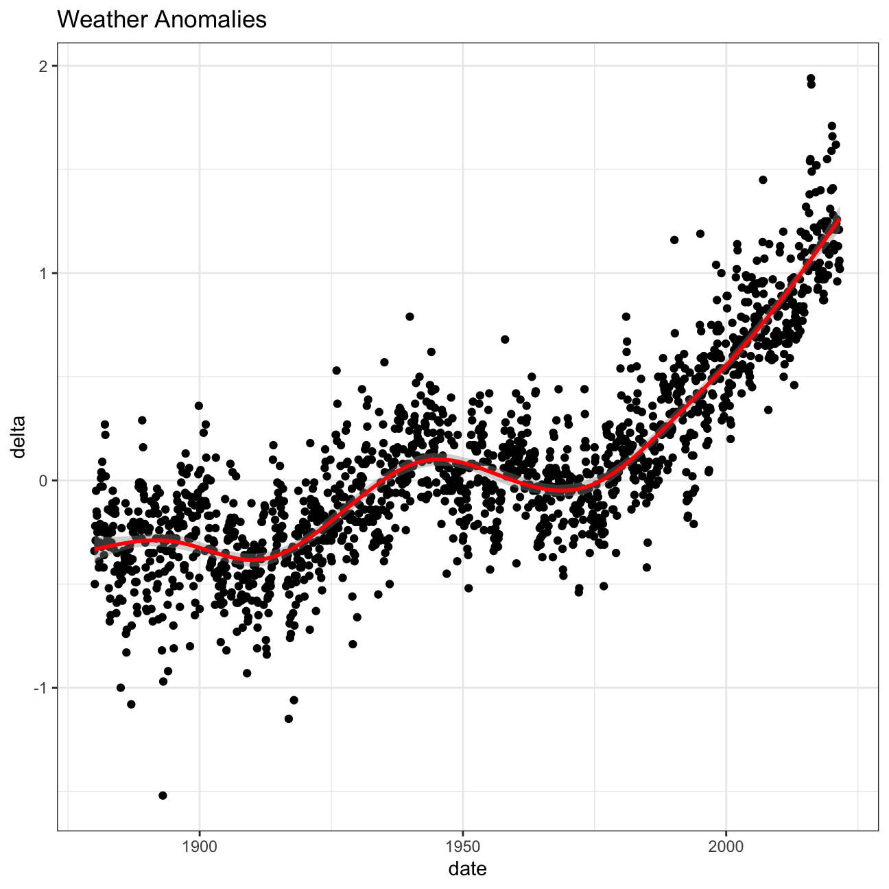
#Now, we can create a scatterplot for our data.
ggplot(tidyweather, aes(x=date, y = delta))+
  geom_point()+
  geom_smooth(color="red") +
  theme_bw() +
  labs (
    title = "Weather Anomalies"
  )

We use facet_wrap to see the weather anomalies by month of the year.

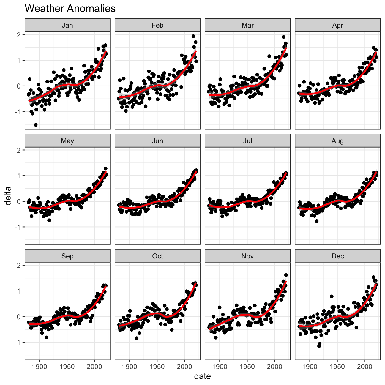
We remove data before 1800 and before using filter. Then, we use the mutate function to create a new variable interval which contains information on which period each observation belongs to.

#We tidy our data further to keep only what we need.
comparison <- tidyweather %>% 
  filter(Year>= 1881) %>%     #remove years prior to 1881
  #create new variable 'interval', and assign values based on criteria below:
  mutate(interval = case_when(
    Year %in% c(1881:1920) ~ "1881-1920",
    Year %in% c(1921:1950) ~ "1921-1950",
    Year %in% c(1951:1980) ~ "1951-1980",
    Year %in% c(1981:2010) ~ "1981-2010",
    TRUE ~ "2011-present"
  ))

Now that we have the interval variable, we can create a density plot to study the distribution of monthly deviations (delta), grouped by the different time periods we are interested in.

#Let's create a plot for the monthly deviations.
ggplot(comparison, aes(x=delta, fill=interval))+
  geom_density(alpha=0.2) +   #density plot with tranparency set to 20%
  theme_bw() +                #theme
  labs (
    title = "Density Plot for Monthly Temperature Anomalies",
    y     = "Density"         #changing y-axis label to sentence case
  )

So far, we have been working with monthly anomalies. However, we might be interested in average annual anomalies.

#creating yearly averages
average_annual_anomaly <- tidyweather %>% 
  group_by(year) %>%   #grouping data by Year
  
  # creating summaries for mean delta 
  # use `na.rm=TRUE` to eliminate NA (not available) values 
  summarise(annual_average_delta = mean(delta, na.rm=TRUE))

#plotting the data:
ggplot(average_annual_anomaly, aes(x=year, y= annual_average_delta))+
  geom_point()+
  
  #Fit the best fit line, using LOESS method
  geom_smooth() +
  
  #change to theme_bw() to have white background + black frame around plot
  theme_bw() +
  labs (
    title = "Average Yearly Anomaly",
    y     = "Average Annual Delta"
  )

1.2. Confidence Interval for `delta`

NASA points out on their website that > A one-degree global change is significant because it takes a vast amount of heat to warm all the oceans, atmosphere, and land by that much. In the past, a one- to two-degree drop was all it took to plunge the Earth into the Little Ice Age.

We construct a confidence interval for the average annual delta since 2011, both using a formula and using a bootstrap simulation with the infer package.

formula_ci <- comparison %>% 
  # choose the interval 2011-present
  # what dplyr verb will you use? 
  filter(year >= 2011) %>%
  
  # calculate summary statistics for temperature deviation (delta) 
  # calculate mean, SD, count, SE, lower/upper 95% CI
  # what dplyr verb will you use? 
  summarise(mean_delta = mean(delta, na.rm=TRUE),
            SD_delta = sd(delta, na.rm=TRUE),
            count_delta = n()) %>% 
  mutate(SE_delta = SD_delta/sqrt(count_delta),
         lower_CI = mean_delta-2*SE_delta,
         upper_CI = mean_delta+2*SE_delta)

#print out formula_CI
formula_ci

# use the infer package to construct a 95% CI for delta
set.seed(1234)

boot_weather <- comparison %>%
  # Choose only  Animation films
  filter(year >= 2011) %>%
  
  # Specify the variable of interest
  specify(response = delta) %>%
  
  # Generate a bunch of bootstrap samples
  generate(reps = 1000, type = "bootstrap") %>%
  
  # Find the median of each sample
  calculate(stat = "mean")

percentile_ci <- boot_weather %>% 
  get_confidence_interval(level = 0.95, type = "percentile")
percentile_ci

## # A tibble: 1 × 2
##   lower_ci upper_ci
##      <dbl>    <dbl>
## 1     1.02     1.11

The data shows us that from 2011 till present, the mean variation from expected temperature is positive 1.06 degree, the standard deviation is 0.276 and there are a total of 132 observations. With bootstrap, we generate a thousand sample means, each calculated with 132 observations extracted with replacement from our dataset, and get a new distribution representing the distribution of the population mean. With 95% confidence, we can say that the true population mean lays in the interval [1.01, 1.11].

Plotting Information

1.2. Confidence Interval for delta

1.2. Confidence Interval for `delta`